
Chapter 5: The impact of per-unit taxes

Per-unit Taxes:
There’s all sorts of interesting taxes in the world. The most relevant in microeconomics are lump-sum taxes and per-unit taxes. Lump sum taxes are where everyone subject to the tax pays some fixed amount. Per-unit taxes are assessed on each unit sold.
A good example of a per-unit tax is the gasoline tax charged at the pump by state tax authorities usually for the purpose of mitigating emissions or repairing damage to the roads. A good example of a lump-sum tax are the fixed user fees charged by several states to owners of electric vehicles. EV’s make different emissions in that they’re heavier and vaporize their tires at a faster rate relative to similar gas-powered vehicles, but the point of the EV tax is to recoup the revenues not paid at the pump for gas, especially given the wear and tear that EV’s still cause on the roads. The good news is that lump-sum taxes are non-distortionary meaning they don’t affect behavior. If you’re paying the same amount regardless, the lump sum tax won’t disincentivize otherwise productive behavior. By contrast, per-unit taxes are distortionary and do generate inefficiency. Much more explanation is necessary and I’ll address the reasons for this inefficiency shortly!
In what follows I’ll focus just on per-unit taxes: This is the situation where a fixed amount such as $1 is added to the price of each unit sold. State and federal gasoline taxes work something like this. There might be a $0.25 per-gallon tax applied to each gallon sold.
In order to analyze the impact of such a tax we make an assumption about whether the tax is imposed on buyers or on sellers. This detail refers to the statutory or legal burden—and is relevant for whether we work on the demand or supply side—and does not have any bearing on whether buyers or sellers actually bear the larger burden of the tax.
Tax on buyers: If a gas tax is officially imposed on buyers (such that it shows up on their receipt) or if a tourism tax is imposed on hotel guests (such that it shows up on their receipt), we would model the tax just as we would with a decrease in demand. We shift demand to the left by an amount equal to the size of the per-unit tax. The reason why is that the consumer is able to afford less of the actual good or service at every possible quantity (their willingness to pay must include the value of the good and the money that goes to the government).
The following graph illustrates a ‘tax on buyers’. I’ve done this with equations so it’ll be easier for you to check. The original demand curve is given by P=10 - Q and the original supply curve is P=2+Q. I’ve assumed there’s a per-unit tax of $2 which means the new tax-inclusive demand curve will be modeled as P=8 - Q which is everywhere $2 lower than the original demand (I’ve measured the same distance between the curves using orange dots in the graph).
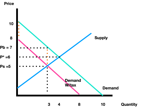
The reason for this is as follows: When we write out an inverse demand curve (the type we graph with price on the vertical and quantity on the horizontal) we use the constant to represent the highest maximal willingness to pay in the market. So P=10-Q implies $10 is the maximal willingness to pay. But if the consumer has send $2 per unit in tax to the government, this becomes: P= 10 - ($2) - Q or just P=8 - Q. The consumer can now purchase goods that they value up to $8 (and then send another $2 on to the government).
Taking a step back to explain the graph, if there were no tax the equilibrium is just P*=6 and Q* = 4. That comes from solving P=10 - Q and P=2+Q as: 10 - Q = 2+Q is 8 = 2Q and then 4=Q, so P(4) = 10-(4) =6 and/or P(4) = 2 + (4) = 6.
Once the tax is applied, the relevant equilibrium for the goods actually traded is where P=8-Q crosses P=2+Q so we have 8-Q = 2+Q or 6 = 2Q or Q*=3 and then P(3) = 8 - (3) = 5 and/or P(3)= 2 + (3) =5. Great, but where does all this fit on the graph?
Once the tax is applied, the demand curve P=8-Q captures the willingess to pay (or marginal benefits) for goods actually consumed. The equilibrium of P*=5 and Q*=3 tells us that’s how much the consumer is paying for goods to the seller, (Ps=5) and how many goods purchased (Q=3). But the consumer actually pays for good and tax, so total price paid by buyers is Pb = 5 + 2 = $7. The government receives tax revenue of $2 x 3 units = $6 for the entire transaction.
Tax on sellers: If a gas tax is officially imposed on sellers (such that the gas station pays the tax perhaps when it acquires the gas from the supplier) or if a tourism tax is imposed on hotels (such that they are reasonable for tracking the number of rooms rented and paying the government accordingly), then we model the tax just as we would a decrease in supply. We shift the supply curve to the left. The reason why is that sellers’ costs are now at least a little bit (artificially higher). It not only incurs the marginal cost of selling another unit of the good or service but also is responsible for paying an additional tax on that unit.
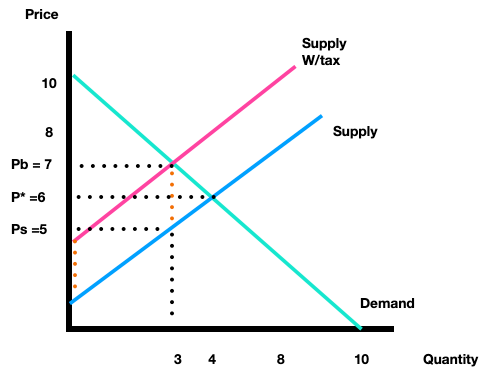
We start with the same beginning demand and supply curves. Demand is just P=10 - Q and supply is just P=2 + Q. Since the tax is on sellers we can leave demand alone and just think of the tax as affecting the seller’s cost structure. Sometimes it’s helpful to think of ‘tax’ as if it’s an ingredient or input in the production process. A change in the price of an important input (from $0 originally, now to $2) will decrease supply which we represent with a leftward shift to: P = 4 + Q. The idea is that the firm’s production costs are captured by the original supply but now the firm must also pay an additional marginal cost of $2 per unit, so we get: P=2 + ($2 tax) + Q yielding: P=4 + Q.
With the new tax-inclusive cost structure we can find the quantity produced and the corrsponding price. P=10 - Q meets P=4 + Q in the new equilibrium: 6 = 2Q or Q=3, then P=10-(3) = 7 and/or P=4+(3) = 7. These are the same as we found above! It has to be! The firm will produce 3 units (Q=3) which come with a marginal cost of production given by the old supply curve MC=P = 2 + (3) = 5, but then has to incur an additional marginal cost of $2 per unit raising the price that buyers need to pay the seller to $7. Of the $7 leaving the wallet of the buyer, $5 cover production costs and $2 go to the goverment. The government receives tax revenue of $2 x 3 units = $6 for the entire transaction.
As mentioned, in either case regardless of whether the tax is on buyers or on sellers, the outcome is the same. Whether we model the tax as on buyers or sellers there will be a difference between the money leaving the buyer’s wallet (or account) and the money entering the seller’s account (when all is said and done). We call this difference a tax wedge. Formally the price paid by buyers minus the price received by sellers, is equal to the size of the tax: Pb - Ps = Tax. In the above example: Pb = $7 and Ps = $5, and we saw the tax was $2.
Importantly we cannot simply add the tax to the original equilibrium price. Notice the original equilibrium price was $6 and despite a $2 tax, the new price of the Q=3 units actually sold in the new tax inclusive equilibrium is $7. The reason why is that we’re dealing with shifts in demand and supply—and the market equilibrium moves accordingly. Because the curves are typically sloped the new equilibrium quantity does not necessarily correspond to a price that’s exactly higher by the amount of the tax. However the original equilibrium price is useful to determining tax incidence—that is, which side is most impacted by the tax. We compare the new price paid by buyers to the old equilibrium price versus the new price received by sellers to the old equilibrium price.
Pb - P* > P* - Ps means buyers are more impacted by the tax and this occurs exactly when demand is more inelastic than supply. Pb - P* < P* - Ps means sellers are more affected by the tax and this occurs precisely when supply is more inelastic than demand. In this particular example, Pb = $7 and P* = $6 and so Pb - P* = $1, half of the tax. Of course also, Ps = $5 and P* = $6 and then P* - Ps = $1, the other half of the $2 tax. In this particular example the tax burden is shared evenly between the buyer and the seller.