


Chapter 6: Welfare Economics
a.k.a consumer surplus, producer surplus, and deadweight loss.

Introduction: Welfare economics is the study of how market participants are affected by market outcomes. We previously introduced comparative statics in the context of the supply and demand model as our approach to studying the effects on the equilibrium price and quantity due to changes in demand, supply, or both. What welfare economics adds above and beyond this existing structure is a way to assess the extent to which individuals are affected economically. We basically are interested in answering the question of how a person or firm’s well-being is affected by market changes.
Foundational principles: Recall we had previously introduced the idea of willingness to pay (consumer’s marginal benefit of the specific unit being consumed). This was measured by the vertical height of the demand curve. In some sense the entire demand curve is comprised of a collection of marginal benefits (one for each respective quantity demanded).
We subtracted the market price from a consumer’s willingness to pay in order to determine that buyer’s economic surplus. For example if my willingness to pay for coffee is $10 and a particular shop sells coffee for $3, my economic surplus as a buyer is $7 if I make that purchase. If we really take our concepts of willingness to pay and economic surplus seriously, I’m actually indifferent between buying coffee for $3 on that occasion and walking right past the coffee shop if someone hands me $7 for free. Either way I come out $7 worth better off. We’ll henceforth refer to this ‘buyer’s economic surplus’ instead as consumer surplus.
Recall we had previously introduced the idea of willingness to sell, or marginal cost, from the perspective of the seller. We said the vertical height of the supply curve measured the marginal cost. And in some sense we could say the entire supply curve was comprised of marginal costs (of the respective quantity supplied).
We subtracted the marginal cost from the market price and that gave us the economic surplus to the seller. If there’s no fixed costs this is actually the same as the firm’s profit. In the coffee example the price was $3 and suppose the marginal cost of producing each additional cup of coffee was $1. Then the shop comes away from the transaction with sellers surplus of $2. If we take our definitions and concepts seriously, the shop is indifferent between this outcome and the situation where I just give them $2 and don’t get anything in return. Henceforth we’ll refer to this seller’s economic surplus as producer surplus.
From the above example we have the following definitions: Consumer surplus is equal to buyer’s willingness to pay minus the market price. Producer surplus is equal to the market price minus the sellers marginal cost. Total surplus is the sum of consumer and producer surplus. Or, equivalently, it’s the marginal benefit minus the marginal cost.
CS = MB - P
PS = P - MC
TS = CS + PS
TS = MB - MC
It’s possible to show the algebraic equivalency between TS = CS+PS and TS = MB - MC:
TS = CS + PS
TS = MB - P + (P - MC)
TS = MB - P + P - MC
TS = MB - MC
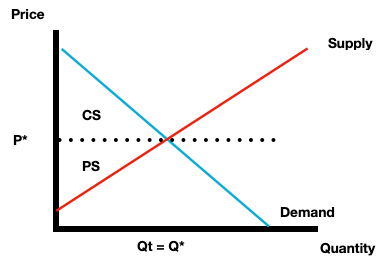
Graphically consumer surplus is the area under the demand curve and above the price, over the units actually traded. Producer surplus is the area under the market price and above the supply curve, over the units actually traded. In the competitive market equilibrium, the quantity actually traded is just the equilibrium quantity. So consumer surplus is the area under the demand curve and above the equilibrium price; producer surplus is the area under the equilibrium price and above the supply curve.
At other prices besides the equilibrium price there will necessarily either be a shortage or a surplus depending on whether the price is below or above the equilibrium. In both cases the area corresponding to consumer and producer surplus won’t extend all the way to the equilibrium because the quantity actually traded will be something smaller than the equilibrium quantity.
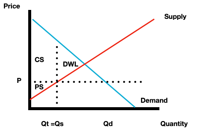
If the prevailing market price is below the true equilibrium price the quantity demanded will be larger than the quantity supplied, a shortage results. The quantity actually traded will be determined by the quantity supplied. That’s because quantity supplied is the limiting factor. People want to buy Qd but there’s only an amount equal to Qs available, so that’s all that gets traded!
Consumer surplus is still the area under the demand curve and above the price, producer surplus is the area under the market price and above the supply curve, and now since the quantity traded differs from the equilibrium quantity we have a new area on the graph, deadweight loss (DWL). This correspond to inefficiency that enters the market. We know this is inefficiency because the area labeled as DWL refers to units for which the marginal benefit to buyers (measured by the vertical height of the demand curve) is higher than the marginal cost to sellers (measured by the vertical height of the supply curve). This tells us that those units are valued more to buyers than they cost sellers to produce…but nevertheless those units are not produced or consumed
Comparing welfare effects: Relative to the competitive equilibrium the buyers and sellers represented by the portion of the demand and supply curves corresponding to the deadweight loss area are worse off. The buyers corresponding to the portion of the demand curve represented by the units still traded (only out to Qt) are better off as a result of the lower price. They get to consume the product, but at a discount! The producers corresponding this portion of the supply curve are worse off. They are still able to find buyers for their product at the lower price but their profits are much lower.