Chapter 6.1: CS, PS, and DWL Example with equations

Demand is P=10 - Q and supply is P=2 + Q.

This section develops an example using equations to describe consumer surplus, producer surplus, and deadweight loss. Here’s the setup: Suppose demand is represented by: P=10 - Q and supply is represented by P=2+Q. Our first step is to find the market equilibrium price and quantity, then to compute consumer & producer surplus and illustrate on a graph. Here’s the equilibrium computation. First set demand and supply equal to find Q*:

10 - Q = 2 + Q

8 = 2Q

4 = Q*

Once we’ve got the equilibrium quantity we need to find the equilibrium price. I always recommend this calculation using both the demand and supply curve to verify. This provides a built-in check step that can help you identify any errors before you proceed. Using demand: P(4) = 10 - (4) = 6 and using supply: P(4) = 2 + (4) = 6, so we know P*=6.

Here’s what this looks like graphically:

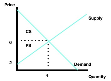
Consumer surplus is the area under the demand curve and above the price, producer surplus is the area unde the price and above the supply. Looking at the graph, clearly we can compute CS and PS as areas of triangles. The formula for the area of a triangle is 1/2(base)(height) so we find:

CS = 1/2(10 - 6)(4-0) = 1/2(4^2) = 8

PS = 1/2(6-2)(4-0) = 1/2(4^2) = 8

Total surplus it the sum of producer and consumer surplus, TS = CS + PS, in this case it’s 16. We know also that deadweight loss (DWL) is zero, because market is in equilibrium! This is our benchmark case, but what happens to CS, PS, and DWL at other prices?

For example suppose the prevailing price in the market is actually P=8 (perhaps due to a binding price floor), then the situation changes. Firstly we know total potential surplus is 16, but since the market will be in disequilibrium we know 16 = CS + PS + DWL in the new example. To actually compute the new CS and PS the first step is to find the quantity actually traded at the price of 8.

Let’s first find quantity demanded and quantity supplied at P=8:

Using the demand curve we know: 8 = 10 - Q, hence Qd = 2.

Using the supply curve we know: 8 = 2 + Q, hence 6 = Qs

We get a surplus because like all above equilibrium price situations the Qs > Qd. Clearly the smaller of the two is the quantity actually traded because even though Qs = 6, consumers only actually want to buy Qd = 2, so 4 units are leftover. We can compute CS, PS, and DWL with this in mind:

CS=1/2(10 - 8)(2-0) = (1/2)2^2 = 2

Let’s look at the graph before we go any further because the area corresponding to producer surplus will be a little more complicated.

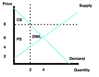
Producer surplus looks a bit like the state of Nevada! It’s an odd shape. But we can still compute producer surplus quite easily if we recognize that PS is basically a rectangle sitting on top of a triangle. Let’s try to calculuate it as the sum of a rectangle and a triangle, PS = Rectangle + Triangle

We for this approach to work we must find the price corresponding to where the rectangle meets the triangle. The quantity coordinate of this point is Qd = 2, we just need to find the price coordinate. We do this using the supply curve which forms the bottom portion of the boundary to PS:

P = 2 + (2)

P=4

Though not drawn on the graph we can envision a horizontal line crossing from the price of 4 through the point (2, 4) that basically partitions PS into a rectangle and triangle.

The area of the PS rectangle is: (8-4)(2-0) = 8

The area of the PS triangle is: 1/2(4-2)(4-0) = 4

So the total surplus is 8 + 4 = 12

But the total potential economic surplus was 16. What’s happened? There’s some potential economic surplus that’s lost due to inefficiency, deadweight loss. If total surplus in the competitive equilibirum was 16 and in this new scenario (with the same equations) is 12, this means DWL is 4.

Total economic surplus in the competitive equilibrium is CS + PS = 16, DWL = 0

Total economic surplus in the disequilibrium/surplus example is CS + PS =12, so DWL = 4.