Chapter 8: Gains from trade

The production possibilities frontier model illustrates the trade-off an economy faces when choosing to produce two goods. We graph the amounts of one good on the vertical and the amounts of the other good on the horizontal. The horizontal and vertical intercepts correspond to the situation where the economy produces only that specific good. The production possibilities frontier is the line that connects the two intercepts. It’s a boundary separating collections of goods, bundles, that are impossible to produce from ones that can be produced. The bundles lying directly on the production possibilities frontier itself correspond to situations where all resources have been exhausted. Bundles closer to the origin involve some degree of inefficiency because there are unassigned resources. Bundles further from the origin and beyond the frontier are impossible to produce with current resources and technology. Here’s an example to illustrate:

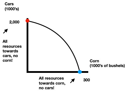
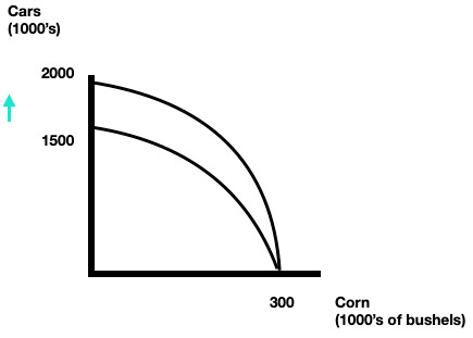
Suppose the economy could produce either corn or cars. If the economy employs all resources in producing cars it is able to generate 2million (and no corn). If the economy employs all its resources in producing corn it is able to generate 300,000 (and no cars). I use these numbers in the graph below but convert the units to 1,000’s so it’s more managable. Note after this scaling that 2million is 2,000 (thousands) and 300,000 is 300 (thousands).

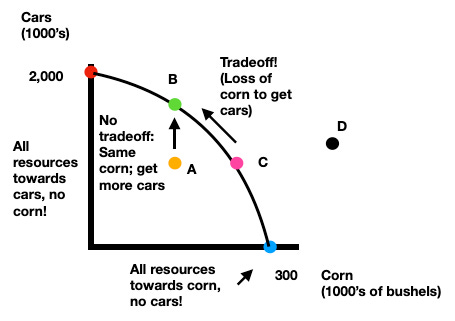
Points on the production possibilities frontier are efficient and points inside the PPF are inefficient. They’re inefficient because not all resources are currently assigned. We can move from an inefficient point to somewhere on the production possibilities frontier without necessarily incurring a trade-off (we just assign some of the previously unemployed resources to producing either cars or corn or both). That’s like going from point A to point B in the graph below (we moved to an outcome where we had more cars and didn’t have to give up any corn). But if we’re currently on the PPF all resources are fully allocated. Moving anywhere else along the PPF requires a tradeoff such as moving from C to B on the graph below (we obtained more cars but this comes at the cost of losing corn).

The slope of the production possibilities frontier captures the relative suitability of the resources to produce each good. The slope of the production possibilities frontier gives us the opportunity cost of producing the horizontal good in terms of the vertical good. Suppose we start at an outcome where we’re producing only cars and no corn. All resources are currently employed towards auto production. If we decide we want to produce some corn we have to redirect some of those resources out of cars and toward corn. First we remove those resources least suited to car production and most suited to corn production (for example, fields and tractors!). In doing so we gain quite a bit of corn while losing very few cars (the PPF is near horizontal at the very top). But as we get closer to the horizontal axis (where everything is going towards corn production) we finally start redirecting resources that are most suited towards producing cars and least suited towards producing corn (for example car factories). This gets us only a little more corn but costs us numerous cars (the PFF is near vertical at the very bottom).

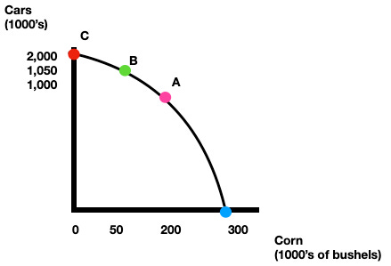
Going from Point A to Point B to Point C gains the economy an additional 50 cars with each step. But the cost in terms of forgone corn is non-constant. From Point A to Point B, the economy loses 100 bushels (from 300 down to 200) but from Point B to Point C the economy looses 150 bushels (from 200 down to 50). This means there’s an increasing opportunity cost (of corn) when trying to obtain more cars.

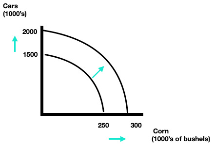
We represent economic growth by shifting the ppf outward. This is a situation where we are able to produce more of both goods.

We represent technological change by shifting out only one intercept. The idea we’re capturing is that the new technology is beneficial mainly to the production of one of the two goods and not directly useful for producing more of the other.

Comparative advantage and absolute advantage:

If we have two traders each producing two goods we can define absolute advantage and comparative advantage. A trader holds an absolute advantage if they are the most efficient producer of that particular good. Basically this occurs when they can either:

1. Produce the most of that good or

2. If they can produce using the fewest resources.

The above refers to two different sorts of examples. (1) If we’re just looking at data over how much stuff each trader is able to produce we can readily identify absolute advantage just by looking to see who produces the most. (2) But suppose there’s a fixed level of output (like painting a room or shoveling a driveway or mowing a lawn). In this case we would identify absolute advantage according to which trader was able to perform the task using the least resource expense e.g. whoever completed the task the fastest would hold the absolute advantage.

Comparative advantage requires a comparison to the other trade and to one’s own other option. Whoever has the lowest opportunity cost of producing a particular good has the comparative advantage in making that good.

Here’s an example:

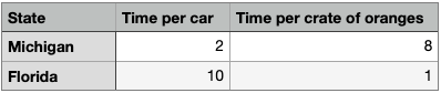
Michigan and Florida can both produce cars and oranges. Suppose it always takes Florida 10 labor hours to make each car and 1 labor hour to make each crate of oranges, while it always requires Michigan 2 labor hours to make each car and 8 labor hours to make each crate of oranges. Further suppose each nation has 80 labor hours available.

Here are those data in table format:

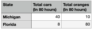
Since we have assumed there are 80 labor hours available we can convert each state’s productivity into actual physical outputs:

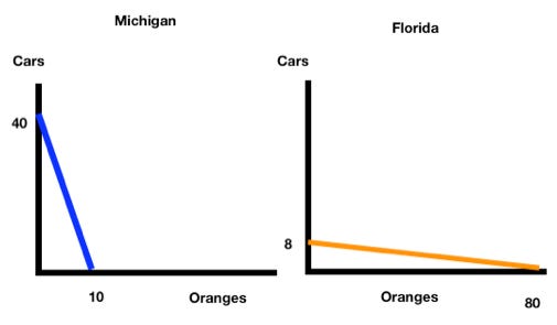
Now that we have physical outputs we can draw the production possibilities frontier for each. We cannot draw the PPF simply from the time requirements to produce each good because the PPF concerns actual outputs that could potentially be created!

In order to determine comparative advantage we have to first compute opportunity costs. Basicaly we must answer the question: What is the opportunity cost of one car for Florida and for Michigan?

• Florida’s opportunity cost of one car is the 10 oranges it gives up

• Michigan’s opportunity cost of one car is the ¼ oranges it gives up

What about for one crate of oranges?

• Florida’s opportunity cost of one crate of oranges is the 1/10 car it gives up

• Michigan’s opportunity cost of one crate of oranges is the 4 cars it gives up

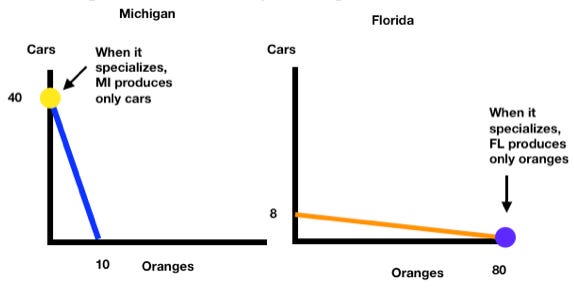
Notice that the opportunity costs are reciprocals! Suppose each nation specializes according to comparative advantage and then trades with the other nation. Florida specializes in oranges and produces 80 crates; Michigan specializes in cars and produces 40. Below I have labeled the bundle each nation produces when specializing:

Are there gains from trade? Sure! These two states will trade at a price that lies between their opportunity costs. So the price of cars must be between ¼ and 10 oranges; the price of oranges must be between 1/10 and 4 cars. Traders are willing to trade when it’s cheaper to obtain the good through trade than incur the opportunity costs of producing it themselves.

Here’s one such mutually agreeable price: Michigan trades 10 cars to Florida and receives 20 oranges. (That’s a price of 1 car to 2 oranges or 1 orange to ½ a car).

Michigan benefits from this trade: 20 oranges would cost Michigan 80 cars! But this trade requires Michigan only give Florida 10 cars. Florida benefits from this trade: 10 cars would cost Florida 40 oranges! But this trade requires Florida only give Michigan 20 oranges.

We can also verify that both agree by checking that the price lies between opportunity costs:

• One car costs: ¼ < ½ < 10 oranges.

• One crate of oranges costs: 1/10 < 2 < 4 cars.

The first inequality tells us that they’ll agree to trade when getting 1 car means giving up between ¼ and 10 oranges. That’s from Michigan needing to give up ¼ a crate of oranges to get a car and Florida needing to give up 10 crates of oranges to get a car. If Florida can get 1 car from Michigan at a price of less than 10 crates of oranges, they’ll be happy!

The second inequality tells us that they’ll agree to trade when getting 1 crate of oranges means giving up between 1/10 and 4 cars. That’s from Florida needing to give up 1/10 a car to get 1 crate of oranges and Michigan needing to give up 4 cars to get 1 crate of oranges. If Michigan can get 1 crate of oranges from Florida at a price of less than 4 cars, they’ll be happy!

I picked these terms of trade because they were nice integers and easy to work with. But there’s many other choices (actually infinitely many) and here are a few other mutually agreeable terms of trade:

-Michigan gets 1 crate of oranges from Florida at a price of 2 cars. (Florida gets 1 car at a price of ½ oranges)

-Michigan gets 1 crate of oranges from Florida at a price of 3 cars. (Florida gets 1 car at a price of 1/3 oranges)

-Michigan gets 1 crate of oranges from Florida at a price of between 1/10 and 4 cars. (FL gets 1 car at a price of between (1/4 and 10 oranges).

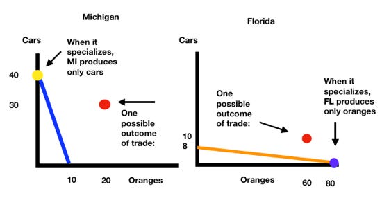
Going back to the original trade, Michigan gets 1 crate of oranges from Florida at a price of 2 cars. (Florida gets 1 car at a price of ½ oranges). Suppose Michigan trades 10 cars to FL and gets 20 oranges in return. If this trade occurs:

• Michigan ends up with 30 cars and 20 oranges (produced 40 cars, 0 oranges but traded 10 cars to FL).

• Florida ends up with 60 oranges and 10 cars (produced 80 oranges, 0 cars but traded 20 oranges to MI)

In this scenario while both are capable of producing cars and oranges, Michigan holds the comparative advantage in cars and Florida holds the comparative advantage in oranges. We know this from comparing opportunity costs. Michigan’s opportunity cost of producing a car, in terms of oranges, is lower than Florida’s (1/4 vs 10 oranges). Florida’s opportunity cost of producing oranges, in terms of cars, is lower than Michigan’s (1/10 vs 4 cars).

They can specialize according to comparative advantage and jointly produce 40 cars and 80 oranges. Then they can agree to trade at mutually beneficial prices. One such price is 1 car for 2 oranges, or 1 orange for ½ cars. They both agree because for Michigan it would cost 4 cars to make 1 oranges itself; trading 1 orange for ½ car is better! Also, for Florida it would cost 10 oranges to make 1 car itself; trading 2 oranges for 1 car is better!

When they specialize according to comparative advantage and engage in mutually beneficial trade, both are able to consume a bundle that they would not have been able to produce on their own (their new consumption bundle is infeasible relative to their own production possibilities frontier!!!)

Here’s a YouTube version of this example: